The Prof Woodhouse lectures on understanding and using SAR data.
A blog series on rediscovering my love of radar remote sensing.
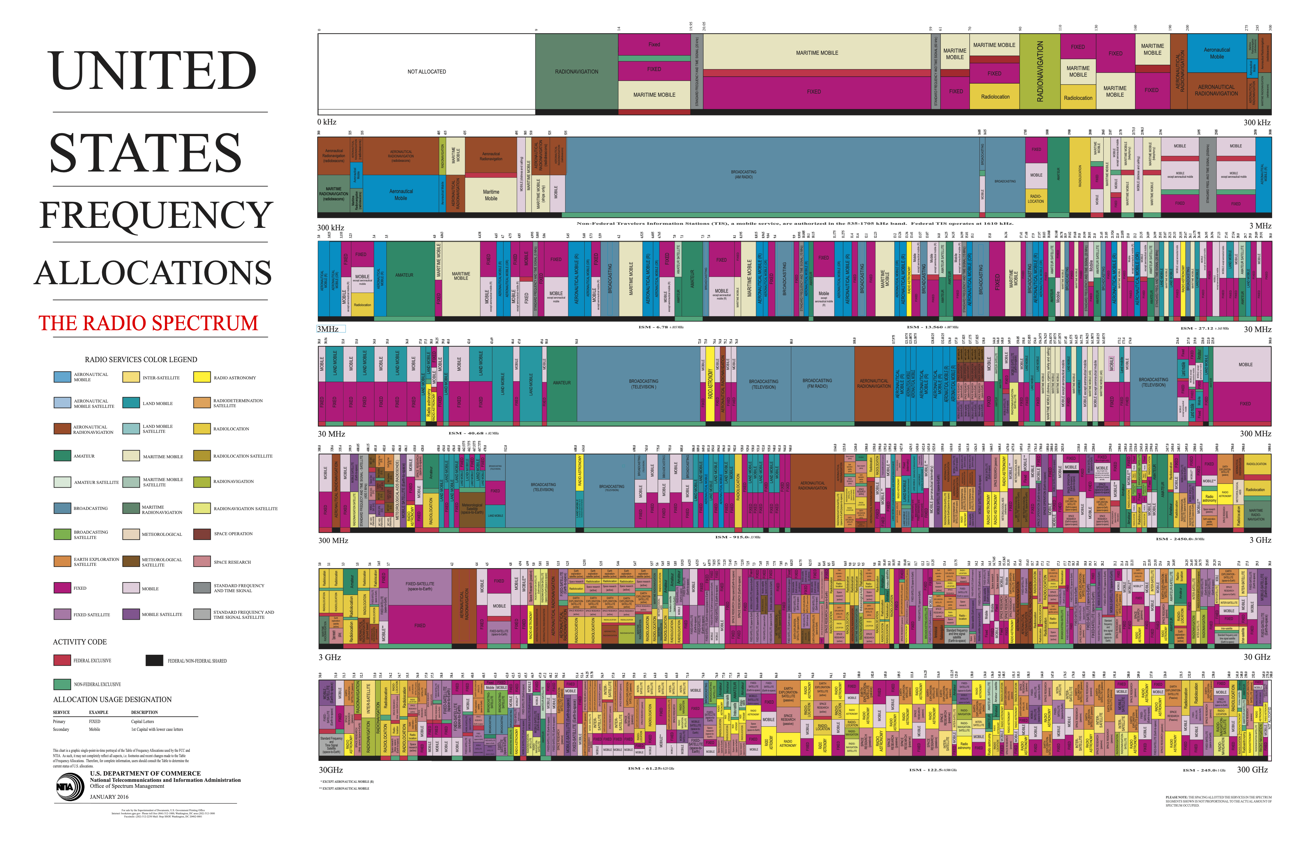 The United States frequency allocation of the radio spectrum (Source: NTCA-USDC).
Here’s a treasure trove of video lectures by Prof Iain Woodhouse, Professor of Applied Earth Observation at the University of Edinburgh and Co-founder of Carbomap Ltd, Econometrica, and Earth Blox, on understanding and using synthetic aperture radar (SAR) data. The video lectures were organised online by the Joint Nature Conservation Committee on November 2020 during the COVID-19 pandemic.
-oOo-
Day 1: Brief history, fundamentals of electromagentic waves, polarisation, combination of waves, some core principles
Take-home messages:
- Radar remote sensing is all about the time dimension
Day 2: How microwaves interact with surface features, surface roughness, moisture content, vegetation
Take-home messages:
- Incidence angle is important! Radar backscatter changes with incidence angle
- ‘Roughness’ is a matter of scale relative to the wavelength
Day 3: How radar builds an image, data properties, unique challenges of radar, speckle, geometric distortions
Take-home messages:
- The P-band BIOMASS mission is one of the most exciting things happening to radar remote sensing. However, one of the key challenges is the spatial resolution due to the limited frequencies in the microwave/radio part of the electromagnetic spectrum that the mission can use. Hence, the spatial resolution would be in the range of 100 meters.
- Saturation levels for AGB: L-band -> 50-70 t ha-1 and P-band -> 150-200 t ha-1, hence okay for regrowth and transition zones
- Why does aboveground biomass saturate? Water cloud model explanation! But also the structural properties of the forest have a big impact on the trend of saturation?
- We know that scaterrers are progressively smaller and more numerous with increasing height into the canopy
Day 4: Practical: how to find data; Split into two groups: SNAP practical and EO browser practical
Take-home messages:
- Speckle is not noise; it is a “noise-like” pattern over homogeneous targets
- A Single Look Complex (SLC) SAR file has two numbers per pixel composed of the amplitude and the phase
- “Looks” — strictly speaking, the number of sub-images averaged to create a final SAR image
- Looks are traded against: spatial resolution (averaging over space such as the Lee filter), and temporal resolution (averaging over time)
- Multilook processing helps get rid of the speckle
- Conclusion from his paper, Woodhouse et al. (2011) in Int J Remote Sens, showed that to resolve ground targets, you could use 3-4 looks if the target has high contrast (e.g., ships that are bright against water that are dark due to double-bounce and surface scattering mechanisms, respectively); however, they suggest using at least 9 looks for lower contrast targets like vegetation
Jose Don T De Alban
carbon markets | redd+ | nbs | conservation | geospatial | land change | sustainability | Southeast Asia