I thought I’d put together some random notes while learning from the Synthetic Aperture Radar: Hazards course taught by Dr Franz Meyer, the Chief Scientist of the Alaska Satellite Facility and Professor of Radar Remote Sensing at the Geophysical Institute at University of Alaska Fairbanks, through edX’s massive open online course platform.
My main motivation for enrolling in the online course was to refresh my foundational knowledge and understanding of polarimetric synthetic aperture radar (PolSAR), and enhance my skills on utilising more advanced techniques including interferometric SAR (InSAR), polarimetric interferometric SAR (PolInSAR), and SAR tomography (TomoSAR)—all of which are quite very exciting technologies to employ in my research.
To anyone else other than myself reading this post however, these notes might not really make any cohesive sense but I suppose each snippet would still be a valuable nugget of information for learning about synthetic aperture radar.
-oOo-
Module 2: Introduction to Synthetic Aperture Radar Remote Sensing.
On the electromagnetic spectrum and the properties of microwaves.
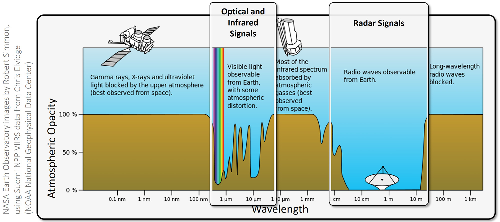
An image of the electromagnetic spectrum that explains the weather-independence of radar imaging. This is a fantastic graphic showing the ‘radar window’ where imaging radar systems utilise a window of high atmospheric transmittance to achieve surface imaging capabilities even during cloud cover. In contrast, notice the variable atmospheric opacities for the visible/optical and shorter infrared wavelengths, and the poor transmittance thereof of other parts of the EM spectrum such as the gamma/x/ultraviolet rays, most of the longer infrared signals, and long-wavelength radio waves. The image would be a good addition in my slidedeck for future talks on the topic too.
On geometric distortions in SAR images.
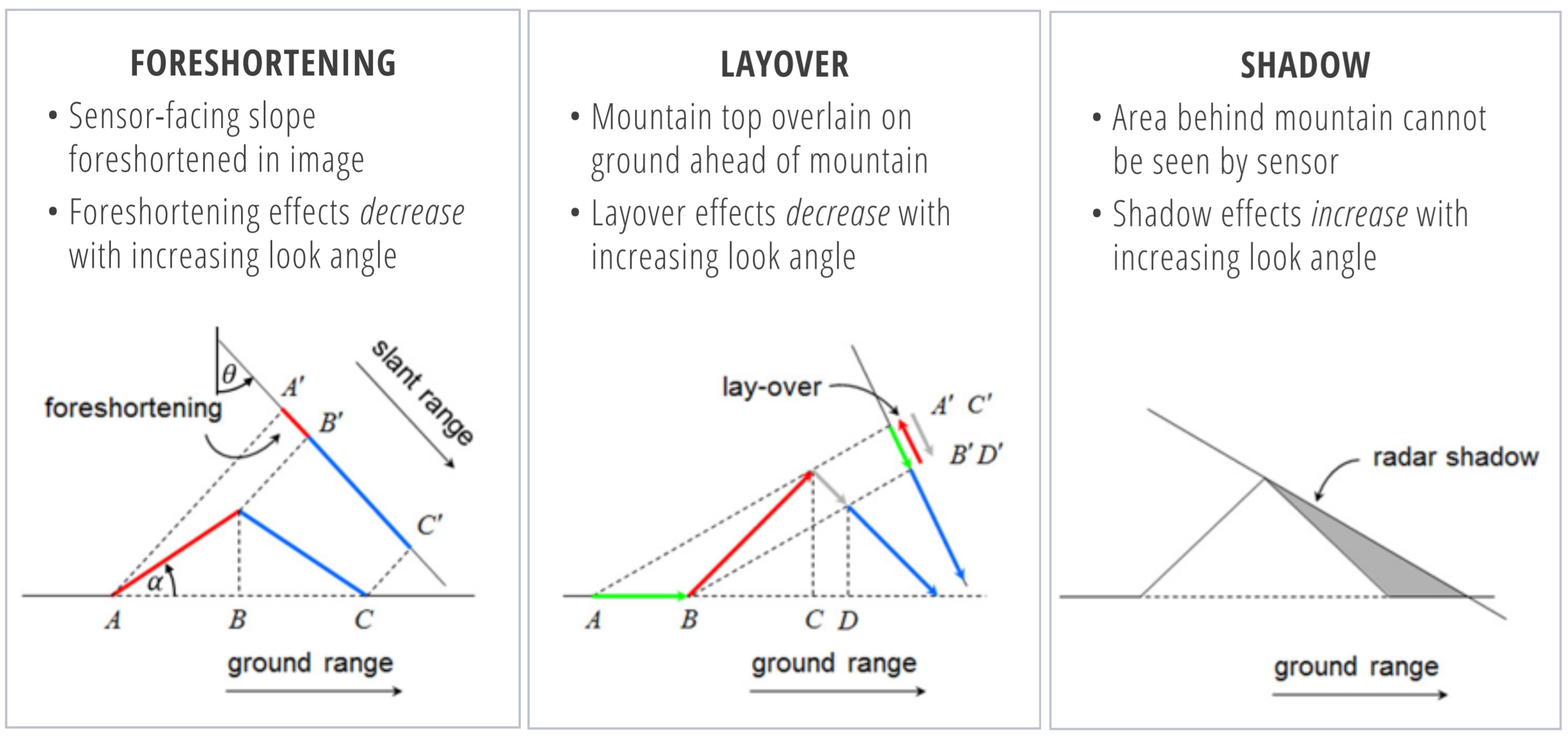
The typical geometric distortions in SAR images due to the oblique observation geometry inherent to all imaging radar systems.Important note: Both foreshortening and layover can be reduced if the look angle θ is increased; however, larger θ will produce more image shadow. Hence, topography-related image distortions cannot be entirely removed, and image acquisitions from more than one vantage point may be necessary to jointly minimise all three imaging effects.
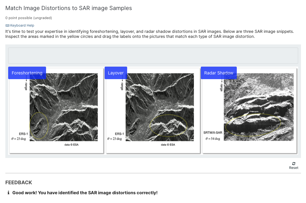
Match image distortions to to SAR image samples. Well, it seems I did well on visually matching the image distortions to the respective SAR image samples.
On geometric and radiometric terrain corrections.
The impact of geometric terrain correction on the appearance of a SAR image. So, which effects did geometric terrain correction (GTC) processing have on the SAR image artifacts? Foreshortening was corrected and mountains now look symmetric and in the geometrically correct location. A number of pixels were also moved to map the SAR image to the correct geographic location.
Example of the results of geometric and radiometric terrain corrections (GTC, and RTC, respectively) on a geometrically distorted image. GTC processing removes the geometric image distortions. Notice the mountains that used to appear as if leaning, now appear symmetric as the position of image pixels is corrected to coincide with their correct geographic locations. Then, RTC processing corrects for the topographic shading in the image, removing the over-brightening of sensor facing slopes.
On radar brightness for different scattering types.
Radar brightness as a function of target characteristics. The image above was acquired by the L-band SAR sensor on the NASA Soil Moisture Active Passive (SMAP) mission. HH-polarisation data are shown. The area covered includes large parts of the Amazon rainforest and Amazon basin in South America. Different areas have vastly different radar brightness depending on their characteristics, particularly (i) open water surfaces are smooth and appear dark in the image; (ii) rough surfaces in bare soil and meadow-dominated areas have low radar brightness; (iii) areas with more significant vegetation are brighter due to increased surface roughness and volume scattering; and finally, (iv) inundated vegetation appear bright in this image, as the L-band radar signals can penetrate deep enough to sense the water under the vegetation canopy.
On radar brightness and signal polarisation.
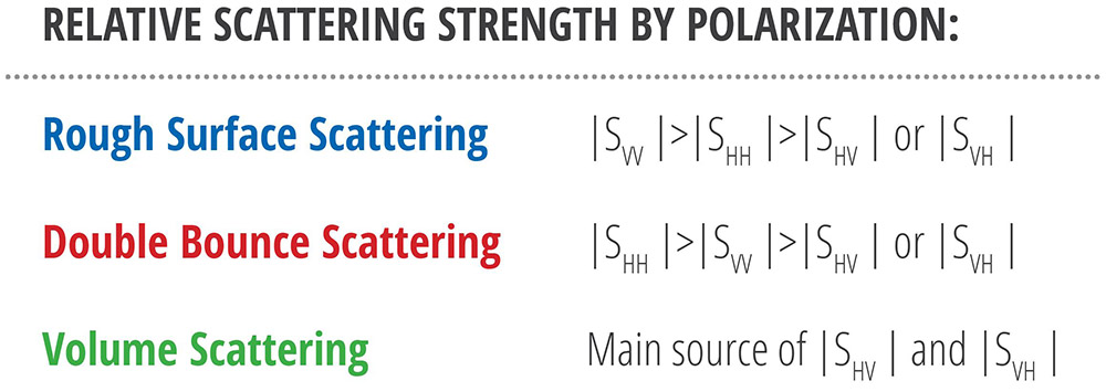
Polarimetric scattering rules of thumb. Scattering types do not contribute to all polarimetric channels equally. Instead, each polarimetric channel ‘prefers’ certain scattering types such that the scattering power |S| in the individual polarimetric channels follows the scheme shown above. These general rules should help when comparing the radar cross-section in different polarimetric channels, which can be applied to perform an automatic classification of scattering types if data with all relevant polarisations (i.e., quad-polarisation data) are available.
On polarimetric signatures for different environments.
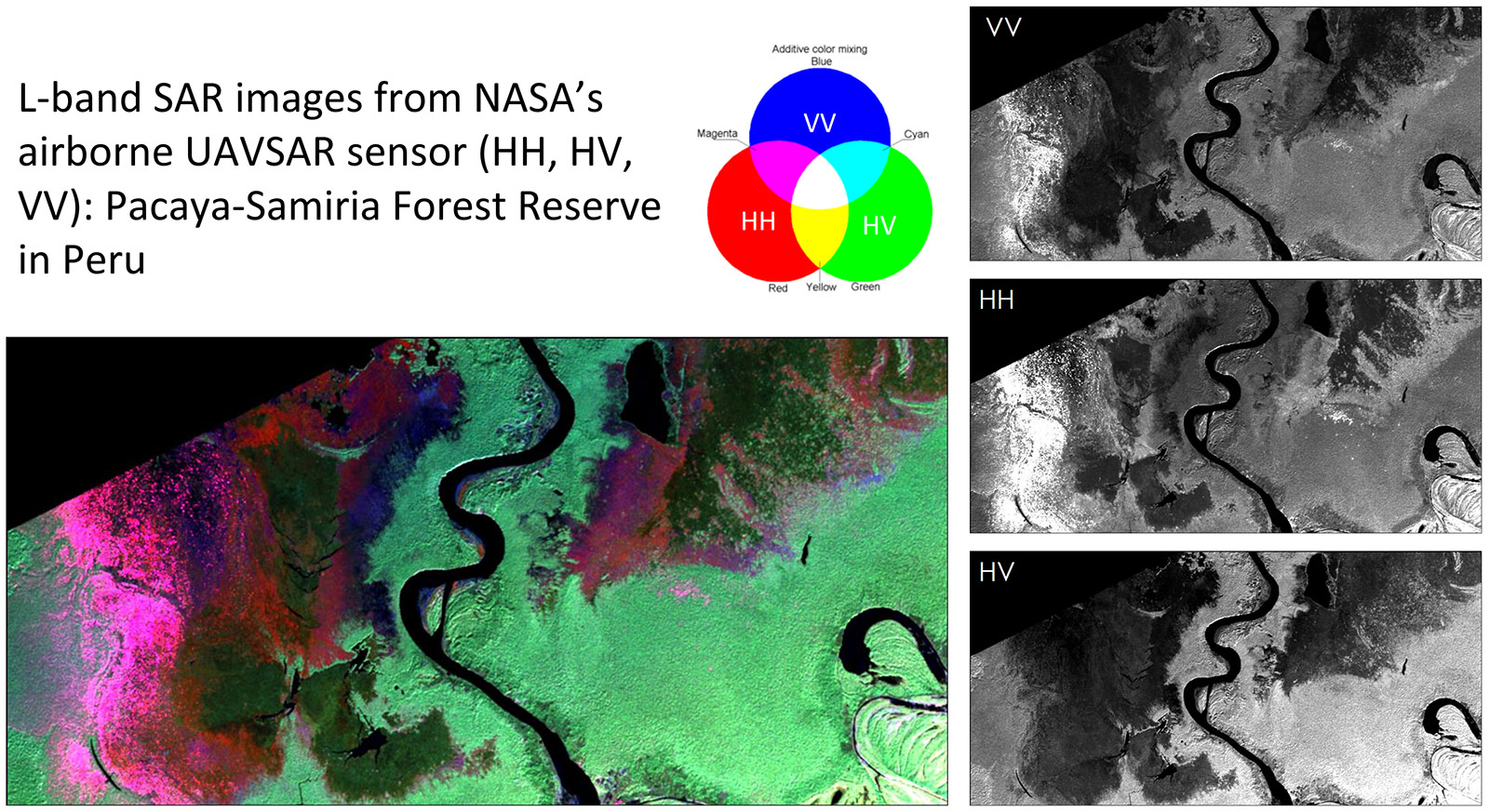
This example over the Pacaya-Samiria forest reserve in Peru demonstrates how different environments have different polarimetric scattering signatures. On the right, the individual SAR images acquired in VV, HH, and HV polarisations are shown. On the left, an RGB composite of these images is shown where the VV band is displayed as blue, the HH band is used as the red channel, and the HV band is shown in green. Some signatures of note: (i) green signatures indicate dense vegetation (HV), where extensive areas appear green in the RGB composite. The strong HV scattering in these areas is caused by dense vegetation; (ii) dark blue corresponds to open water (VV), where smooth open water appears dark with a slight blue hue caused by slight surface roughness on the water surface; and (iii) red and pink patches show inundated vegetation (HH), where inundated vegetation shows enhanced double bounce scattering (scattering of smooth water and tree stems). Slight surface roughness is mixed in with the areas showing a pink hue.
Module 3: Introduction to Interferometric SAR.
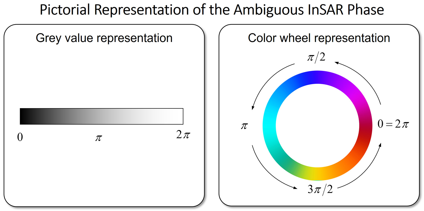
On representing the interferometric phase.
Pictorial representation of the interferometric phase. The color wheel is more appropriate for representing the ambiguous interferometric phase than the grey-value scheme because the color wheel is better for distinguishing small phase variations.
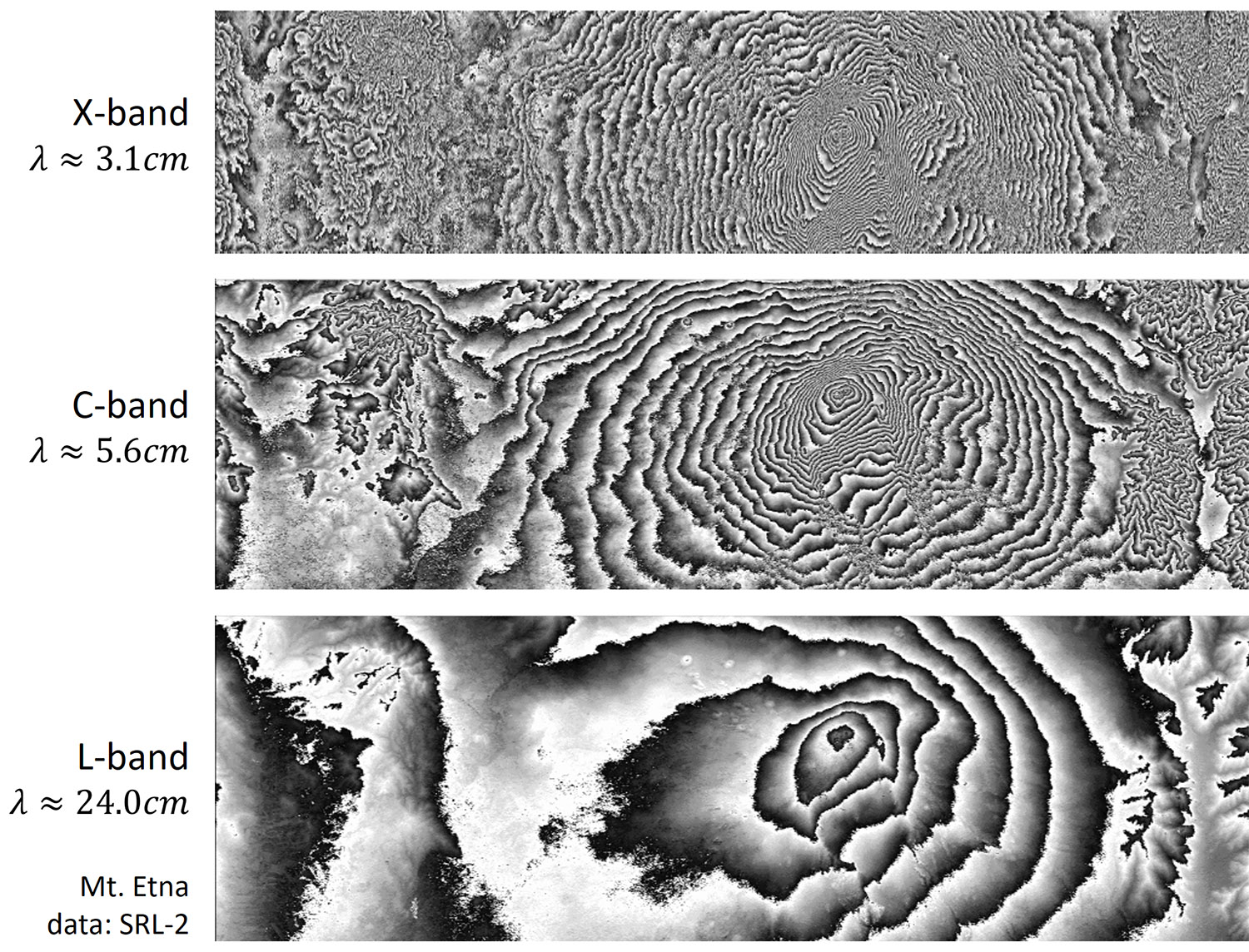
On measuring and mapping topography from InSAR.
Interferometric sensitivity to topography as a function of sensor wavelength. For a constant perpendicular baseline, the accuracy of the topographic height improves for shorter sensor wavelengths (i.e., all things equal, X-band sensors provide better topographic accuracy than L-band sensors). In the image, the three interferograms of an undulating terrain differ in the sensor wavelength used, but have otherwise identical imaging parameters including the perpendicular baseline, slant range, and look angle. It can be seen that the fringe density progressively increases as the wavelength decreases from L-band (24 cm) through C-band (5.6 cm) to X-band (3.1 cm). The higher fringe density at shorter wavelengths indicates higher sensitivity to topography, yielding more accurate topographic information.
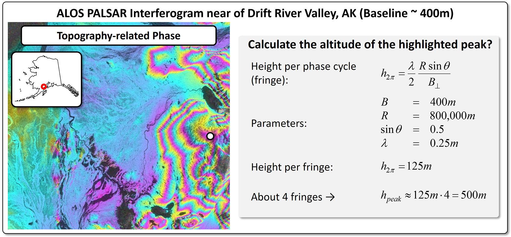
Topographic mapping with InSAR. The interferogram in this image was collected from two ALOS PALSAR L-band SAR acquisitions over a coastal area in southwestern Alaska, USA. You may note a few things: (i) regions on the left side of the image have rather homogeneous and very slowly varying phase (the color of the phase map changes slowly). This is due to a rather flat topography in this area; (ii) fringe patterns can be seen on the right side of the phase map. The rate at which phase is changing (fringe density) reflects the local surface slope. Areas of steep slopes are represented by tighter fringe spacing. More gently sloped areas have broader fringe spacing; (iii) about 4 fringes can be counted between the left side of the image and the area marked by the white circle. The math on the right hand side of the figure shows that this translates to an approximately 500 m height difference between the coastal areas to the left and the area marked by the circle. The good and bad of interpreting interferograms: So the interferometric phase pattern gives you an immediate sense of local topographic slopes. Despite that, the ambiguity of the phase makes it difficult to immediately measure the differences in topographic height between two points in the image. We needed to count the ‘fringes’ (phase cycles) between these points using phase unwrapping to arrive at differences in topographic height.
On differential InSAR and deformation monitoring.
The concept of differential InSAR. Satellite orbits rarely repeat themselves exactly, and in all likelihood, the interferometric pair will show a non-zero baseline. The interferometric phase is very sensitive to surface displacement as the displacement-related phase component can capture displacement signals at fractions of the sensor wavelength. To utilise this tremendous measurement capability, however, the displacement-related phase component needs to be extracted from the interferometric measurement displacement-related phase component by performing DInSAR processing.
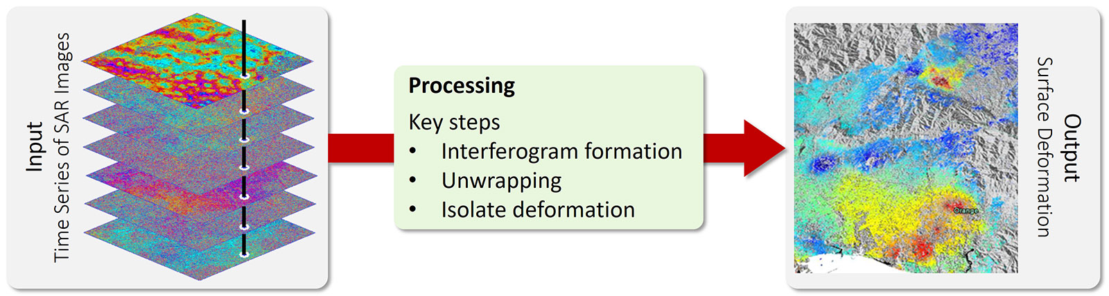
Differential InSAR processing. DInSAR processing attempts to remove the topographic phase from the measured interferogram with the goal of isolating the surface displacement and facilitating precise surface deformation mapping. Removing the topographic displacement can be done in several way, with two of the more common approaches entailing: (i) the utilisation of an existing DEM, which is used along with the known satellite locations to simulate and subtract topographic phase components from the measured interferogram; and (ii) the formation of many interferograms from at least 3 SAR acquisitions such that if these interferograms have different spatial and temporal baselines, a system of linearly independent equations can be formed and solved to arrive at an estimate for surface topography and surface displacement rate.
On the limitations of single-pair InSAR techniques.
InSAR limitations brought by phase decorrelation. The main limitations of InSAR relate to phase decorrelation (amount of decorrelation: X-band > C-band > L-band) and atmosphere-induced distortions of the interferometric phase. The 12-day Sentinel-1 interferogram time-series over Sierra Negra volcano on the Galapagos Islands demonstrate both limitations. Several fringes related to surface uplift can be observed near the center of the image. However, the interferograms also show time varying phase screens caused by the atmosphere and areas of significant coherence loss, which are more prevalent in highly vegetated environments. Both of these main limitations can be partially mitigated using advanced InSAR time series techniques.
Module 4: InSAR Time Series Analysis Techniques.
On the motivations for InSAR time series analysis.
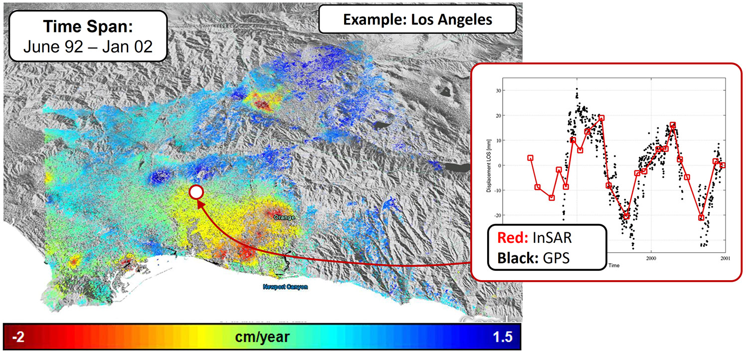
Motivations for InSAR time series analysis. The image above showcases how InSAR time series analysis is able to reveal variable surface deformation in the Los Angeles area induced by groundwater extraction. There are two compelling reasons to move from traditional InSAR (based on a single image pair) to InSAR time series analysis. First, InSAR time series analysis enables the study of temporarily extended (and varying) phenomena such as many surface deformation phenomena that develop over time. A comparison to GPS (above image) demonstrates the high accuracy InSAR can achieve while exceeding the capabilities of GPS in the spatial sampling of the phenomenon of interest. Second, InSAR time series improves the precision with which surface displacements can be measured. As most deformation phenomena develop slowly, we can exploit the redundancy in InSAR time series stacks to mitigate noise and nuisance signals such as atmospheric effects, residual topography, and decorrelation.
On the goals InSAR time series analysis.
Goals of InSAR time series analysis. One of the goals of InSAR time series analysis is to improve the extraction of displacement-related phase components from the observed interferometric phase. This is achieved by exploiting the different temporal, spatial, and baseline dependencies of the displacement (or surface deformation), and the atmospheric, topographic, and noise-related phase components. A large number of interferograms is formed to separate these different phase components based on their respective characteristics.
On approaches for InSAR time series analysis.
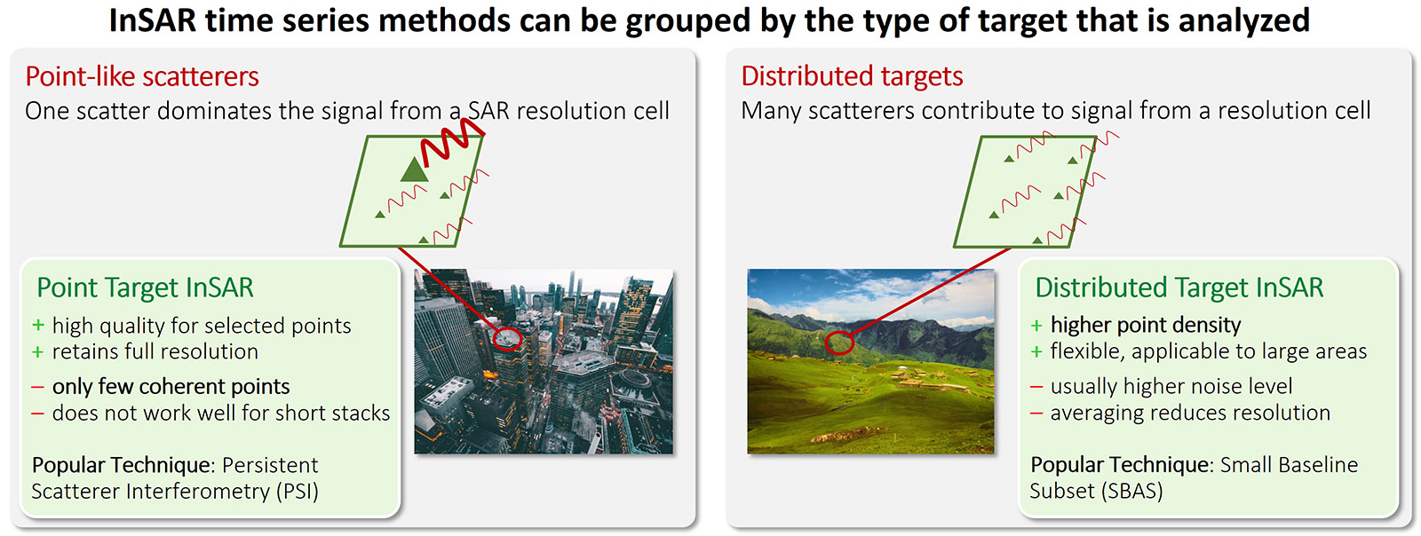
Point target vs distributed target InSAR. There are two types of InSAR time series analysis methods. Point target InSAR such as Persistent Scatterer Interferometry techniques utilise the often superior scattering stability of point-like scatterers to track deformation through time. Point-like scatterers—individual scatterers that dominate the signal from a resolution cell—are often remarkably stable over time, making them ideal objects for deformation monitoring. The famed scattering stability is due to the fact that point-like targets are often associated with stable man-made structures such as buildings, poles, corners. Point target techniques provide high quality deformation information at point target locations. However, the density of point-like scatterers is often low, resulting in a sparse distribution of usable points. Distributed target InSAR techniques utilise distributed targets for deformation monitoring, which occur in natural environments (meadows, fields, bare soil) where many similarly bright scatterers contribute to the information in a resolution cell. Distributed targets are plentiful, facilitating densely sampled deformation maps. However, deformation measurements on distributed targets are often of lower quality and require spatial filtering.
On the high phase stability of persistent scatterers.
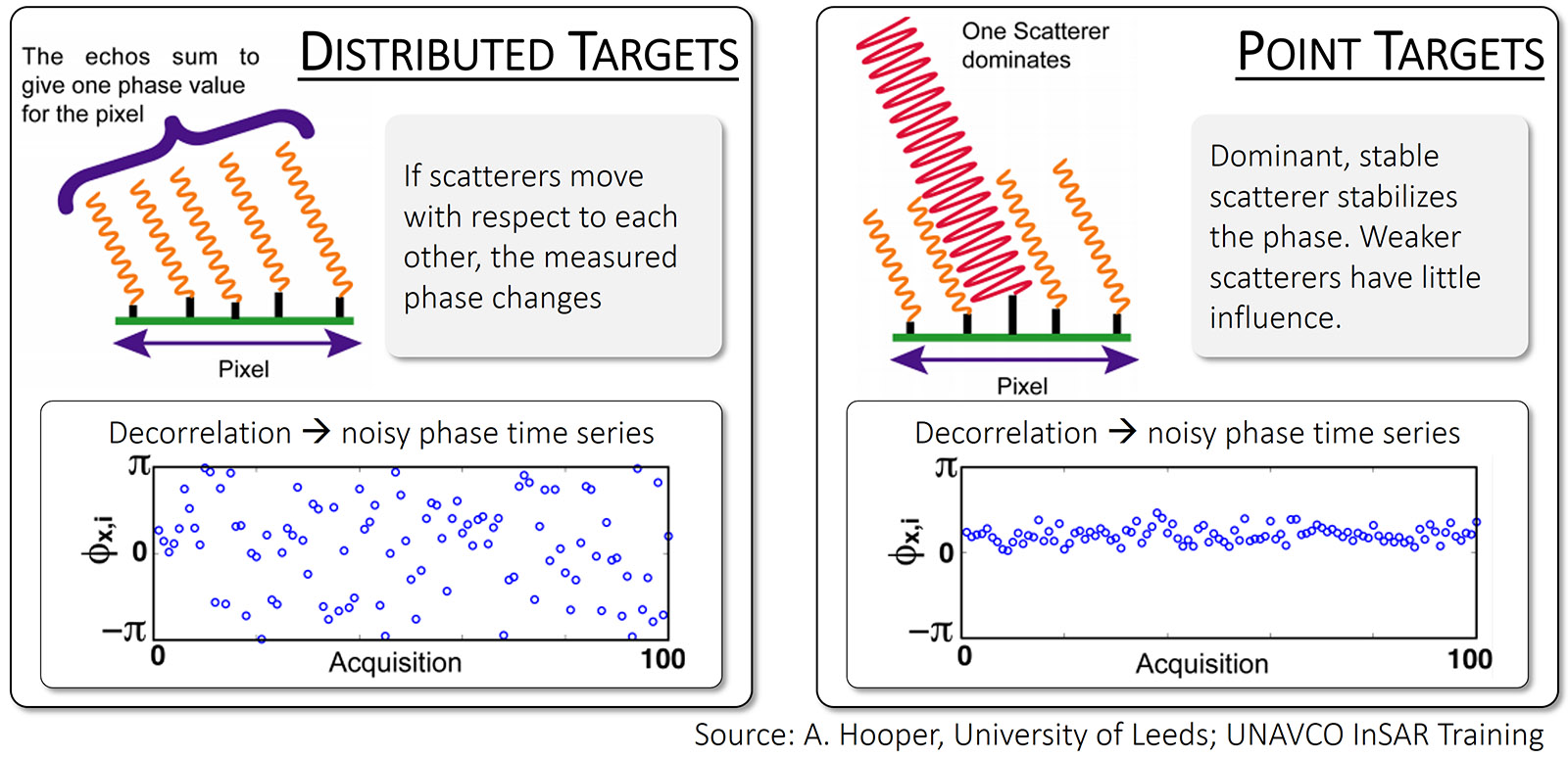
Why do persistent scatterers have high phase stability? The phase of distributed targets (left image) changes quickly in time because the relative movement of equally-bright scatterers changes how the scatterers in a resolution cell interfere with each other. On the other hand, a bright stable target (persistent scatterer; right image) in a resolution cell dominates and stabilises the phase measurement, which is ideal for long-term deformation monitoring. Hence, Persistent Scatterer InSAR first identifies PS points in a SAR image stack and then analyses their phases across time for surface deformation analysis.